Z3Help

Introduction

Why another programming language? Don’t we have enough of them?

Well, let us try this real world experiment. Go to the best programmer you know. Pick the simplest formula you can think of: E=mc^2. Ask how the Energy (E) can be calculated, for a mass (m) of 1kg, 2kg, 3kg,… 10kg and for a constant Speed of Light (3x10^8m/s). Let us just watch the programmer for what happens next. Yes, go ahead and start a stop watch!

It is likely that the programmer would pull up a spreadsheet, and type formulae notations into the document such as on the right, and within a minute or so, give you the answers.

C	=3*10^8
M
1	=D5*$E$3^2
=D5+1	=D6*$E$3^2
=D6+1	=D7*$E$3^2
…	…
=D12+1	=D13*$E$3^2
=D13+1	=D14*$E$3^2

Or maybe, the programmer would make a program, in some computer language to do this, and will come back to you in about an hour!

Today, an ordinary computer can do billions of operations per second! And even with the best techniques, translating from our human language to computer language takes minutes or hours even for the simplest of equations! This clearly shows the biggest problem with the current state of the art computer human interaction.

That is why we created a simple language for you and the machine called:

z^3

The vision behind the z^3 language is specifically to make human interaction with computers convenient, simple and elegant, at any level of complexity, all immersed in a framework of immense power.

What is Z^3

z^3 is a general purpose language that is easy to write and natural to read, powered by high performance, scalable, computing constructs which unlimits thinking and expression. z^3 console is launched from ZCubes platform on any HTML5 enabled browser.

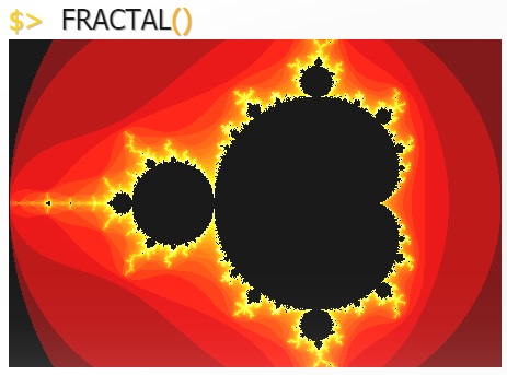
FIGURE 1 - FRACTAL PATTERN GENERATED BY USING Z^3.

In the following sections of the document, z^3 specifics will be described in easy to follow examples.

ZCubes Platform

ZCubes is a platform for users to create and manipulate information. The website address is http://www.zcubes.com. To load the application simply click on the Z icon, or directly visit it at http://www.zcubes.com/zspace/zcubes.aspx. z^3 console is launched by clicking the icon on the bottom right of the ZCubes platform. Please refer to Appendix 1 for operators, symbols and notations used in ZOS.

Being an omni-functional platform, ZCubes allows creation of documents with unparalleled power, with almost any imaginable functionality provided at your finger tips. Upon load, the ZCubes Platform looks as below with a simple minimal interface: Menu items can be accessed by clicking the Z button.

ZAP is the desktop version of ZCubes that allows deeper access to programming interfaces than the web version. The methods to access z^3 in ZAP is similar to the web-version.

The ZOS Console to interact with z^3 can be accessed using the command console button at the extreme right bottom. Commands can now be typed into the Enter ZOS Command area as indicated below.

Entering command like 1..10@SIN and pressing enter gives you the result in the window.

ZCubes Selected Features

ZCubes is a 3D platform, which changes its nature based on the user's perspective.

For example, it can function as a blackboard in one moment, and a presentation tool in another moment, or a spreadsheet in yet another moment.

The platform changes like a chameleon based on the attributes users wish to have anytime. More details on how to work with ZCubes is explained in section 8.

Data Collections

An array is a simple data structure to create, collect and manage data. z^3 transforms conventional arrays into something much more powerful called Sets.

Sets

Sets are new data types used in z^3. These are arrays (not necessarily rectangular) that are flexible in size, shape, types and contents, which make them extremely powerful. The term set is italicized throughout the document for easy identification.

The following are notable properties of Sets, compared to conventional arrays:

•Sets are unstructured arrays, or varied sizes and types.

•Sets may contain other Sets of any complexity.

•Sets are enhanced with several member functions(A listing of these are given in Section 8.5 Appendix V Member Functions) in z^3.

For example, sets can be printed out with the built-in member function print(), to get the internal representation in z^3.

Set-based z^3 resolves complexity and scaling issues, while achieving high-performance, extreme flexibility or natural expressiveness.

Set - Simply a collection of data

Let us start with a simple example.

At the ZOS Console, right after the command prompt indicated by $>, enter the command 1..3. Let us use the member function .print() to display the set representation in z^3.

The “two dots” operator used in 1..3 creates a simple set, with 3 integer elements (1 at index 0, 2 at index 1, and 3 at index 2 positions). Sets have indexes starting at 0, which is a common practice in C-like languages.

Once a set is created, various operations can be performed on it. As you shall see later, the results of many of these operations are also sets, which mean we can continuously apply these operations until desired results are achieved.

An interesting point to note is that the set 1..3 can be implicitly declared without any extra word or punctuations unlike most languages(Several Series Generation Techniques are detailed in Appendix IV Series Generation).

It is also important to see the use of .. operator as a technique to create a sequenced collection of number values (from lower end 1 to upper end 3 - in this case as a range). To create a set filled with a series, the [ ] operator is not required. Hence, whenever we use [ ] array operator along with .. operator, it indicates a set of set(s). This is effectively a set with index 0 containing three elements (this inside element being similar to the array in Example 1..3.print()).

This is clearer when we apply .print(). 3.

In the example above: the internal set representation is displayed as 1,2,3 .

A set can contain other sets (containing any type of data) recursively (or one within the other without limits), as in the following,:

In this example more complex items (including a set) is collected into one set: Location at Index 0 contains integer 2, at Index 1 contains integer 4, at Index 2 contains a set, and at the location at the last Index 3 contains integer 2.

Sets created can then be operated on using functions (or even sets of functions) using the @ operator as shown below:

However, aggregate functions such as SUM should be applied to the entire array, not to each element.

In the example above, the result may appear confusing at first, since SUM function is applied for each set element, if we use the @ operator.

The following example shows the application of function SUM() to a set (not separate elements). The three elements of set are added, resulting in 6, the expected answer.

Let us see another operator … (“three dots”) in action.

The “three dots” notation generates a set with 4 values, as a geometric series from 1 to 8 as 1, 2, 4, 8. Another example below shows geometric series from 1 to 30.

Now let us look at more complex scenarios.

In the following, the “two dots” (..) operator is compounded to make an even more powerful expression:

Here the first .. indicates a series from a start value to an end value, and the second .. is used as an increment operator. Hence, the result includes all numbers from 1 to 10, with an increment of 2.

Set- Object Representation

In z^3, {} is used for the creation of object data structures (also known as associative or composite set (4.g)). The JavaScript associate array syntax and semantics are kept as they are.

In this Example, a set with two items (a as a set of 3 integer values, and b with another set of 4 integers) is dynamically created.

By simply using = (as assignment operator), A is defined as a variable, which now stores an associative set, which can then be referenced as below.

Now A.a refers to the attribute a of the newly created variable A. Likewise, A.b will display the contents of item b of variable A.

Set-Complex Set Layouts

Now, consider a simple set of three elements (equivalent to 1..3):

A more complex layout of a similar set is given below, where 1 and 2 are in one element (stored as a sub set) of the new set.

In the below Examples show slight variations on how non-regular layouts of set elements can be defined.

These examples clearly demonstrate that using clear and elegant operators in z^3 (such as .. and …), simple, consistent and powerful structures can be created.

Matrix – as a Set of Set(s)

Arguably, a matrix (which can be represented as a Set of Set(s)) is one of the most frequently needed and useful data structures in programming.

A table can be visualized as an example of a matrix – such as a table containing rows and columns in a database, or a simple table with rows and columns in a simple document or the tabular grid(s) in spreadsheets.

In mathematical terminology, matrix definitions and usage are very common - such as identity matrix, diagonal matrix, sparse matrix, and so on. Hence,

operations on matrices are provided by z^3 using a rich set of operators and functions.

Matrix Operator(||)

Matrix construction can be done with the || operator.

For example, creation of a 4x4 identity matrix can be done with the following simple notation:

|4| as it is displayed above gives a 4 by 4 identity matrix by definition.

Note that the matrix operator || is used here for both matrix declaration and initialization.

If only one dimension is given, it is assumed that the matrix requested is an identity matrix.

This highlights the simple and minimalist style provided by z^3 throughout. Similarly, |4,2| constructs a 4x2 matrix.

Similarly, |4,2,2| constructs a 4x2 matrix, with each cell having 2 values, all initialized to zero:

The variations of matrix construction can be seen in the following examples.

The notation inside matrix definition can be with commas, the letter x, or a simple space.

A square matrix of 2 by 2 with initial values 0, is given by this notation.

Here a square matrix of 3 by 3 with initial values 0 is obtained. Similarly, you can define |4x2| or |2x4| as given below.

Now, let us look at some more advanced examples.

The example above gives a zero-filled 2 by 2 by 2 matrix (i.e., a matrix of 2 by 2, with each element containing a zero-filled 2-element matrix).

The following gives a zero-filled matrix of 2 by 2 with 3 elements each.

The matrix notation can scale-up for more complex uses, and for any size and level of dimensions.

Set input to functions

The simplest case is SUM of set 1,2,3 is calculated by the following:

In the following Example, the set 1..3 and 2..4 are passed to the function SUM, and it gives the sum of all the numbers in both set. Compare this later, against the combinatorial arguments applied to functions (detailed in Section Combinatorial Arguments below).

The following Commands, calculate the SUM of all parameters (each of which may be a set containing a series) provided in each case.

We can have any number of arguments to aggregate functions.

Commas and parenthesis can be omitted for simpler calls. For more complex calls, commas and parenthesis may be required to avoid ambiguity. However, it is always recommended use the brackets to avoid confusing situations.

|| Binary Operation

The binary operation with matrix operator | |, called the “two bars” operator, is simple and natural to use.

Two matrices of compatible sizes can be operated on with matrix operations, such as |+|, |-|, |*|, and |/|, as given below.

Also the two bars of this operator can brace any arbitrary function or operator. The below Examples show combining of two matrices using a simple function represented with x and y, provided in between the | | operator( x and y represent variables from sets on each side of the binary operation. x and y can be replaced by any two names for the variables).

Member Functions of Set

A variety of useful and powerful member functions (listed in 8.e Appendix V Member Functions) are provided for sets. Examples include, .print, .$, .index, .tenth, .random, etc.

By convention, member functions are generally in all lowercase, while primary functions are generally in all uppercase. These member functions are invoked using dot-notation, like most conventional object-oriented languages.

For example, .transpose() is a member function that will return the transpose of the matrix.

With the simple notation above, a 3x3 matrix is created, and filled with random numbers up to 3. The following shows the use of .fillwith() to fill the dynamically created matrix of size 3x3.

Note that in the case above all cells are filled with 8, and in the case below a series of numbers from 1..9 are used.

Again, matrix dimensions can be given implicitly (such as |2| for a |2x2| matrix).

Functions like random(), deal(),and many other available functions listed in the Section 8.e Appendix V Member Functions can be used to manipulate sets.

creates a 3 by 3 set and fills it with random numbers with values upto 3.

The .fillwith() member function is used to fill a 2 by 2 matrix with numbers 3, 4, 5, and 6.

The member function det calculates the determinant of a Matrix.

Note that the simple function DET() and det() also can be invoked to calculate the determinant of a Matrix.

The statement above will calculate the determinant of the matrix A1 created in the previous step (Example: A1=|2x2|.fillwith(3..6)).

The .across() member function of set is powerful way to operate on two matrices, cell by cell. The result of this operation applies the operation among EVERY combination of cells among the matrices(This is similar to the TENSOR product of matrices. Here it simply provides the row column .index() as result).

Even when we graduate into more complex combinations of computational constructs, the language keeps its fundamental simplicity and consistency. Looping construct is rarely needed in z^3, as functions can be applied iteratively with implicit initialization (and increments) in a natural order and minimalistic style.

While set and functions can be used in very rich ways with z^3's syntactical simplicity, traditional programming language syntax and style also can be used. This is beneficial for backward compatibility and for creating clever new possibilities of mixing traditional and newer styles.

@ Applied To Operator

To apply a function or set of functions to a set of values, we use the APPLIED TO operator, indicated by @.

gives you a list of SIN(x) values for input ranging from 1 to 360.

The @ operator can be a powerful ally when mixed with the concept of Combinatorial Arguments detailed below.

Combinatorial Arguments

The @ operator differs from a simple call of a function on a set with a simple twist. The @ operator treats input data set as Combinatorial Set.

That is, in [1..4,2..3]@SUM, the SUM function is applied to COMBINATIONS of values in the two sets, namely [1,2,3,4] and [2,3] (denoted by 1..4 and 2..3).

Note that this is not the same as the set [[1,2,3,4],[2,3]] being treated as input to the SUM function. The following example makes this clear:

Every combination from each set 1..4 and 2..3 are paired as parameters into the SUM function in the listing above. This powerful function enables users to avoid loop-in-loop constructs that are often seen in C-like programming

(e.g., for i=1..4 and for j=2..3).

By extension, combinatorial arguments can be extended to inner loops of ANY depth (i, j, k, l, m, … etc)

We can also reverse two sides of the @ operator, as given below where the function SUM is applied to the combinatorial data given on the right, giving the same result as above Example.

Compare this with Example SUM(1..3,2..4), which is similar but with simple application of SUM to the full set of input, without any combinatorial loop.

Applying Combinatorial Set to Set of Functions

In z^3, data sets can be collected into any number of set or combinations, and applied to any number of functions.

It does not matter whether data or functions are given first.

The following examples shows this expressive power of z^3, with data and/or functions separated by comma, which behaves as a list operator.

The inputs are generated and applied in a natural order iteratively. This makes z^3 keep its readable form, without needing a lot of complex looping expressions.

Simple Function Representations

Functions can be made on the fly using expressions within quotes as given below (example: "x^2+5*y")

Here, the data set on the left are passed to the set of functions listed on the right.

In the functions that are expressed as strings such as in ("x^2+67*y") in the above Example, the symbols x and y represent the first and second of the combinatorial arguments.

This feature allows users to express content of a function in the most natural manner, without complex function declaration decorations.

Easy Multi-Line Representation of Z^3 Code

Note that code can be split into multiple lines (using the Shift+Enter key) in the ZOS platform editor, as given in the below Commands.

The examples above indicate .merge() member function, that operates on two sets (one on the left, and one as a parameter), merged with the functions listed as second parameter of the member function.

In the below Example, .rand() function fills the set created using the ARRAY function. Then the across() operation takes each such cell combination from each matrix, and then applies the list of functions [SUM, AVG] given as the second parameter.

The partial output is given below.

Using || as "Such That" Boolean Expressions

We can check a set against logical expressions, like in the following examples:

Here, the range of values is tested for a logical conditional test, to give truthiness of the check in a simple set series.

In the above Example 62, the set 4..8 is passed on to the check x>5. The result is a Boolean set of true and false.

In this above Example, 1..100 is passed on to the check x>5. The result is the value itself or 55, based on the result of the check on each specific element.

It is possible to compound conditions in a traditional sense easily with logical operands like && (and logical check) as follows:

Associative Set/Composite Set As Objects

Object instances can be expressed easily using simple implicit notation. There is no need for explicit constructors or definitions as may be required in conventional object oriented languages.

A1 is an instance of Object, with initial values given, in lines with Object-Oriented (OO) terminology. The qualification of members (whether it be a value or a function) is coded with traditional (.) operator. The result is an object meant for further processing, hence the display shows [object, Object]. However, members of this object are now accessible using A1.a. For example:

It is also possible to use member names in quotes as indexes, as given below:

The following example demonstrates these properties:

The qualified member is used as an argument to a function:

Assignments are straightforward. The type of the variable value is taken implicitly from the right hand side (RHS) value.

The variable represented by the left hand side (LHS) name, is dynamically recast to the type of the assigned new value.

For example, in the object A1, c which was initialized as a string before, can now be used as a place holder for a function:

The output indicates that this is a function with a single parameter a.

Now the A1.c represents a function, which can be called as given below.

Similarly, b in A1 can be assigned to the SIN function with no extra coding:

Now, we can call A1.b as a function, which then gives the SIN value of 30, in radians.

A similar example of object assignment and member access is given below.

The members can be qualified with the initial LHS ids for reference, as usual:

<<< MEMBER ASSIGNMENT OPERATOR

Assignment of attributes of an object can also be done using <<< operator.

Please note that B1["apple"] can also be expressed using B1.apple, like in conventional javascript.

GLOBAL ASSIGNMENTS USING <<<

The following example demonstrates the use of attribute assignment operator <<< to assign a set of functions to an attribute of an operator:

Now this assigned a global variable called orange, that now contains a set of functions SIN and COS.

Please note that SIN and COS take input in radians. DSIN and DCOS take input in degrees.

This set of functions in orange is applied to a set of numbers 1..4, in the below Example.

Also note that orange is now a global variable in the environment for easy use (as a set or collection of functions, which then becomes a powerful object to use to apply multiple functions at once).

Functions

In most languages, a function like SIN takes one input and gives a scalar output. In z^3, the same SIN function behaves in more powerful ways. If given a scalar SIN will give a scalar result like other languages, but if given an arbitrary set of inputs, z^3 will give a similar set of outputs. Now, more interestingly, functions can be: (1) Simple member functions of a set, as in objects as member functions, or (2) Set of functions, that provides an elegant organization.

Set of Functions

It is possible to use the expression in (below Example) as a one line computation, or decomposed into multi-line computation (Commands A=[ "x^2", "x*2", "x+2"] and 1..4@A).

The example below, demonstrates the declaration of three functions, each with one parameter x, collected as a set and assigned to A for easy reuse.

In z^3, the data provided to such sets of functions can be a set (or set of sets) of any breadth and depth.

The set of three functions are now invoked on a range of values 1..4 below:

Note that explicit looping constructs are avoided. The logic represented by the set of functions is applied to each data value in a sequence 1..4.

This style of applying a set of data to a set of functions demonstrates z^3's functional approach (i.e., writing WHAT is to be computed, and hiding HOW it is computed).

The built-in FOREACH function (same as FOR function) can also be used to achieve combinatorial arguments and set of functions in a straightforward manner(Since lowercase for is a standard keyword in some platforms, FOREACH function is provided to side-step any conflict in case of case-sensitivity).

It is clear that the data set given as arguments are used from left to right(Any extra parameters are simply ignored, while using the matching values to compute the functions). The first set 1..2 behaves as the outer loop index values, and the secondary set 2..4 behaves as the inner increments, for x and y values respectively, which are associated from left to right.

As the following example clearly demonstrates that FOREACH is a rich function that takes data set in multiple forms, and sets of functions collected in a set:

The parenthesis and commas can be dropped as in the previous example, if it would not cause a syntactic ambiguity.

Simple Reusable Function Declarations

A function can be declared as follows:

Instantly, a function Y1 is created, with parameter u, t and a, with parameter(Global variables can be accessed from the inside of simple function definitions. However, to keep simplicity of variable names in local scope, any global variable up to 3 characters in length referenced inside the body of the function would need an _ (underscore) prefixed to its name) names which are automatically detected by z^3, in order of their appearance.

On the other hand, if an uppercase name is used, it is assumed to be a global variable than a parameter. This name can be used in the parameter list if an _ is added to the name. (For example, A=M_*cat; will have M_ and cat as variables, but A=M*cat will only have cat as the variable).

If there are similar names existing in the environment, z^3 will rename the function.

Combinatorial Arguments

The following gives an example of series and combinatorial arguments being used to replace the use of a spreadsheet to do such calculations!

Let’s check what would happen if more data values were provided as parameters, than that were defined in the function Y1 (which expects only 3 parameters u, t and a).

As expected, the fourth parameter value 8 is ignored and the computation is completed with the first three parameters of the data set.

Data can be simply listed following the function with a space as a separator as below.

If the user prefers to list the data in a parenthesis, data may be listed with a comma (,) operator as a separator.

Consider an example of counting of PRIMES, up to a certain number.

With z^3 notation, we can repeat this process for any set of numbers.

In the example below, series of odd numbers (from 1 to 10) are created, and the count of primes that are within 1 to that number are then calculated.

The ranges can now be expanded from 1..10 to 1..100000..10000, demonstrating powerful ways of combining z^3 notations to achieve complex expressive calculations, without sacrificing simplicity and scalability..

Set $, $$, $$$ and $_ Member Functions

A set of functions can be invoked in every element in a set by using the powerful .$(dollar) member function.

In this case, four even numbers are generated by the EVEN function, which are then incremented by 2.

1..5.$("1/x") 1 0.5 0.3333333333333333 0.25 0.2

The above output lists the reciprocals of numbers 1..5.

Remember that .$ is not quite the same as .map functions that you may be familiar with, since .map operations only operate on the children in the first level of the array or set. On the other hand, .$ operates on every element in the set, recursively.

The result of .$ is also a set, and can be fed into further member functions to operate on, such as SUM shown above.

Now, consider the following command to add numbers from 1 to 10.

The member function (.$_) (dollar-underscore) can be used to apply an aggregate function (such as SUM) to the entire set, resulting in a single functional result.

1..10.$_(SUM)

The member function (.$$) (dollar-dollar) applies the set of functions provided on each row (by row) of the set.

The member function .$$$ (dollar-dollar-dollar) function works along columns, compared to (.$$) that operates on rows. 1..10.$$$(SUM)

Set Functions and Set Programming

The use of sets as collections of statements and function calls creates an interesting possibility of program segments that is self-explanatory.

The above function definition creates a function when called gives the input a and b, as well as the result, all as ONE set in the output!

This creates the possibility of holding data sets that carry inputs and outputs of a process for reporting uses or further analysis. Such composites create a rich expression possibility for calculations in z^3.

Here, the results shows inputs 1 and 2 (a and b in the set program), followed by the array of results from the the computation of the set of functions [SIN(a),COS(b),SIN(b),COS(a)] in the set program.

Such functions defined as set, gives unique expression power to programmers. In the example in Command V(1,2), the input is effectively carried along with the output.

Let us consider some powerful ways to create functions.

The function F1 is now defined, and calling it is simple.

Another example that demonstrates the expressive power:

As can be clearly seen above, the outputs carry the inputs as well as the results, creating absolutely interesting possibilities of handling data, as well as avoid unnecessary complexity in programming.

This effectively creates a function F3 that can add up series between a and b, of any interval c.

The sum of 1+3+5+7+9 is obtained as 25 by calling F3 with the parameters 1, 10 and 2.

The following shows another interesting use of set Programming, coupled with || function definition (Section 4.e). 118. $> 1..4|[x^2,x^3]|

Here the function [x^2,x^3] itself is a set. The result of this set function is applied on the series 1 to 4. The result is a 2 dimensional set of such combinations of output.

Advanced computation of lists

Trigonometric calculations are useful in a wide varied domains, such as electrical engineering,map projections etc. These require computation of lists.

Series of values thus generated are heavily used during further computation, as inputs, as well as loop control variables; but most languages fail to support quick and easy generation of common collections and series.

z^3 makes the generation of such lists incredibly easy, starting with x..y..z notation such as in 1..10..3.

Generation of commonly used angles, in radians or degrees, can be easily achieved as given below.

More examples and details of Series Generation are given in Appendix IV Series Generation (8.d).

The series computed can be used as in cases like:

Series computation

The design of z^3 attempts to provide natural language interfaces, with terse and powerful notations.

Hence SUM 1..4 can also be implied by the following natural language expressions.

1 to 4 implies all numbers from 1 upto 4 (i.e., 1, 2, 3 and 4).

Note that this is not the same as ADD 1 4 which should give the result 5.

A series by an increment can be expressed using the x to y by z notation.

Built-in Functions in z^3

z^3 has powerful prebuilt function libraries. This collection is continuing to grow daily; and already these number into the thousands.

These range from functions in Mathematical, Statistical, Financial, Engineering, Medical, Database, and many other domains.

Several of these standard library functions are documented at http://wiki.zcubes.com

Consider some interesting available functions.

Permutations and Combinations

Permutation relates to the act of arranging all the members of a collection into some sequence or order; whereas Combination is a way of selecting items from a collection, such that the order of selection does not matter.

z^3 comes with functions to list permutations and combinations of items, as well as techniques to count and list them.

All possible permutations of 1, 2 and 3 are shown above.

All possible permutations of 1, 2 and 3, in sets of two elements, are shown above.

All possible combinations of 1, 2 and 3, of one element are shown. Next, all possible combinations of 1, 2 and 3, of two elements are shown.

Common Number Series

EVENS is a function that returns x even numbers, for a requested x.

The series thus generated can be input to functions as SUM, or vice versa.

The following creates a jagged collection of 1, 2, 3 and 4 even numbers.

Simple Number Stats

STATS is a powerful function that applies a lot of Statistical Functions on a series of numbers.

Let us look at a larger collection of numbers.

It scales-up for more complex needs easily, by considering the STATS function call for 1, 301, 601, and 901 in a series:

Now, Example FOR(1..10..2 "COUNT(PRIMES(x)))" is scaled below to a larger range of data. 135. $> FOR 100..1000..300 "COUNT(PRIMES(X))"

z^3 scales-up to handle larger range (though limited by your computers capacity), as shown in the following computation:

136. $> FOR 1...10000000 "COUNT(PRIMES(X))"

Note the “three dots” operator between 1 and 10000000, which signifies the generation of a geometric series.

Please try:

FOR 1...10000000 "COUNT(PRIMES(X))" as a first attempt to test the capacity of your device.

Set Operations

Several operations are provided to operate on sets.

Some examples with set-theoretical operations are given below:

z^3 Simple Examples

z^3 language, while being based on global standards, is unlimited in scope by being open to extension. It does not take a single approach to problem expression and solution, but many approaches, which result in highly flexible possibilities of terse and verbose expressions based on user skill and style.

Several example real-world problems are described in sections below.

Sets and Related Structures

Matrices

Set (or sets of sets) of complex dimensions can represent conventional matrix definitions in an effortless manner. z^3 provides a collection of powerful matrix functions and manipulation capabilities.

Matrix Generation

With z^3, a wide variety of matrices can be generated with ease.

In Section 4.c (Matrix Operator(||)), generation of a simple set is described. For example,

|4,2| generates a simple 4x2 matrix.

Known types of matrices of required size can be generated using the MATRIX (or MATRIXWITH) function. For example, it is very common to fill a matrix with “positive”or “zero” or “negative” values as needed as follows:

A matrix of size 4 of positive integers is generated below.

Another example of a matrix of size 4 of negative integers is equally easy.

Similarly, a matrix of 4x4 size of integers.

Similarly, a matrix of 4x4 size of Boolean values (0 or 1).

More special matrices can also be generated as described below .

Hilbert Matrix

The Hilbert matrix is a square matrix with entries being the unit fractions.

For example, H_i,j = 1 / i+j-1. So, 2x2 Hilbert matrix is

1	1/2
1/2	1/3

For n, it is a square matrix nxn with the values as

1, 1/2, 1/3, 1/4, . . ., 1/n

1/2, 1/3, 1/4, 1/5, . . ., 1/n-1

1/3, 1/4, 1/5, 1/6, . . ., 1/n-2 . . .

1/n, 1/n-1, 1/n-2, . . ., 1/2n-1

In z^3, simply calling MATRIX function with arguments “hilbert” and size will provide the result:

Hermitian Matrix

Hermitian Matrix (or self-adjoint matrix) is a square matrix with complex entries that is equal to its own conjugate transpose, that is, the element in the i-th row and j-th column is equal to the complex conjugate of the element in the j-th row and i-th column, for all indices i and j: In mathematical representation:

a_ij= a_ij or A^T=A

Here is an example:

Hankel Matrix

The Hankel matrix (or Catalecticant matrix), named after Hermann Hankel, is a square matrix with constant skew-diagonals (positive sloping diagonals), e.g. A_i,j=A_i-1,j+1

Toeplitz matrix

The Toeplitz matrix or diagonal-constant matrix, named after Otto Toeplitz, is a matrix in which each descending diagonal from left to right is constant. The Hankel matrix above is closely related to the Toeplitz matrix (which is an upside-down Hankel matrix).

A_i,j =A_i+1,j+1=a_i-j

For instance, the following matrix is a Toeplitz matrix in z^3:

Hadamard Matrix

Named after the French mathematician Jacques Hadamard, a square matrix whose entries are either +1 or −1, and whose rows are mutually orthogonal, is called a Hadamard Matrix.

In geometric terms, this means that every pair of two different rows in a Hadamard matrix represent two perpendicular vectors.

In combinatorial terms, it means that every pair of rows have matching entries in exactly half of their columns and mismatched entries in the remaining columns.

Vandermonde Matrix

Vandermonde Matrix, named after Alexandre-Théophile Vandermonde, is a matrix with terms of a geometric progression in each row, i.e., an m × n matrix.

In z^3, the following is an example of Vandermonde matrix:

Upper and Lower-Triangular matrix and Symmetric matrix

In Upper Triangular Matrix, all elements under its diagonal are zero. In Lower-Triangular Matrix, all elements over the main diagonal are zeroes. In Symmetric Matrix both sides of the diagonal elements are filled, but with elements around the main diagonal symmetric in value.

The hyphen between upper-triangular is optional.

Pascal Matrix

The elements of the symmetric Pascal matrix are the binomial coefficients, i.e. S_i,j = (n r) =n!/r!(n-r)! where n=i+j,r=i.

In other words: S_ij = i+j C_i =(i+j)! /(i)!(j)!

Matrix Sizes

SIZE function can be used to find the size of sets.

A second parameter can be used to indicate the size is to be obtained in a specific dimension.

The result gives the size along dimensions 0 and 1, of an array of size 4x5.

Matrix Operations

The following code is used to generate a 3 by 3 set filled with 3. The RANDOM function is then called on each of the members using the $ function fills each element with random values within 0 through 3. As you can see MX is then assigned with the result.

The matrix MX is now added along a row using MROWOP using the + operator.

This result is interesting, as much as it is powerful. The true value as the second parameter indicates that the cumulative and running result as each element is operated on (as it applies columns in each row) are listed. Only cumulative result is provided if the third parameter is empty is false.

The same can be done for each column, with the top row indicating the cumulative result, and rows below this row showing results (when each element was added by row to the next element) in the column.

MATRIXPACK splits the matrix into elements of sizes given as parameter. Here it divides matrix MX into pieces of 2 elements.

Matrix Arithmetic Operations

Simple Matrix addition, multiplications, negation, etc. can be obtained using MATRIX related functions such as below. MMULT([1,2,3],[[4],[4],[2]]) 18 Note the use of brackets for the vertical matrix as in [[4],[4],[2]] in the above Example. 1..3**3 is a simple notation to duplicate a set, by a requested number of times, indicated by **. In this case, 1..3 will be replicated 3 times.

MMULT then operates on the two sets as below.

173. $> MMULT(1..3**3,1..3**3) 6 12 18 6 12 18 6 12 18

MMULT, does scalar multiplication of the argument is a scalar, with the matrix that is provided in the other argument.

MATRIXADD conducts simple addition of matrices.

MATRIXNEGATE multiplies each element by -1, or effectively negates the elements.

MEQUAL checks each element in a set to see if it matches a provided value, in this case a 10x10 matrix filled by 2, is checked against 2.

MEQUAL(ARRAY(10,10,2),2)

Vector Operations

Dot Product or Scalar Product of matrices can be conducted on vectors represented as matrices or sets using the DOTPRODUCT (also called SCALARPRODUCT) function.

Similarly, Cross Product or Vector Product of matrices can be conducted on vectors represented as matrices or sets using the CROSSPRODUCT function.

The functions CROSSPRODUCT and VECTORPRODUCT are the same.

Matrix Determinants

In linear algebra, the determinant is a special value associated with a square matrix.

For example, in a matrix that represents the coefficients of a System of Linear Equations, its determinant provides important information about the matrix. The system has a unique solution exactly when the determinant is nonzero; when the determinant is zero there are either no solutions or many solutions.

Determinants occur throughout mathematics. In some cases they are used just as a compact notation for expressions that would otherwise be unwieldy to write down.

For instance, the determinant of the matrix:

|A| has the value as: (2x3x2 + 2x4x2 + 1x1x6) – (1x3x2 + 2x4x6 + 2x1x2) = -24

In z^3, the determinant of a matrix A is denoted as det(A), det A, or DET(A).

In z^3, determinants of any size square matrix is easily calculated, as for the matrix x below (generated using deal member function).

Determinant of an identity matrix is 1, as indicated in the below Example.

The determinant of a randomly generated 3x3 matrix is given below. 186. $> det(deal|3x3|) 0.02381843917684589

Matrix Rotations

Matrix rotation can be achieved by the MATRIXROTATE function.

A simpler z^3 notation for the same is given below, using member functions.

Simple Matrix Merging with Functions

Here two 10x10 sets, filled with 10 are merged cell by cell and the result is merged together.

To enter lines with soft line-break, use Shift+Enter, instead of simple Enter.

It makes it simple to provide member functions indented under the main object as given above.

Across Matrices Merging with Functions

In z^3, .across() member function is a powerful operation that applies a specific function or set of functions on each pair of elements on the two input matrices.

Consider a simple 3x3 identity matrix.

The .across() function applies SUM to the two identity matrices.

A more powerful example of applying a set of functions (SUM and AVG in the following case) on the each combination of elements of input matrices is shown next.

Quick Multiplication Tables

Consider the following use of the across function to generate a Multiplication Table in Command 195.

In this case, the .across function is used in such a way as to operate on every pair of numbers between 1 an 10. This is a simple demonstration of the .across operation, (which can also be used on an array of functions as indicated previously) to create useful collections of results, such as those that can be used for contour plotting etc.

Using the power of sets, you can get the multiplication factors of any one number (using the [ ] element accessing capability). For example, the following command gets the multiplication table for the number 6 (note the 0 based indexing of sets as used).

Puzzles and Other Interesting Computations

There are several special problems and puzzles that are pre-solved in z^3 for enthusiasts, to analyze various case scenarios and to slice and dice such results.

Magic Square

In recreational mathematics, a Magic Square is an arrangement of numbers (usually integers) on a square grid, where the numbers in each row, the numbers in each column, and the numbers in the forward and backward main diagonals, all add up to the same number.

A magic square has the same number of rows as it has columns, and in conventional math notation, "n" stands for the number of rows (and columns) it has. Thus, a magic square always contains n^2 numbers, and its size (the number of rows and columns it has) is described as being "of the order n".

The smallest nontrivial case, a 3 × 3 grid that is a magic square of order 3 is shown next.

In z^3, magic squares of any size can be created using the MAGICSQUARE function.

The sum of every row, column and diagonal, which should be a constant value, is called the Magic Constant or Magic Sum, M. Every normal magic square has a unique constant determined solely by the value of n, which can be calculated using this formula:

$M={\frac {n(n^{2}+1)}{2}}$

The row wise and column wise sum of the magic square elements show that for an m of 4 rows and columns, 4*(4^2+1)/2 = 34 would be the magic constant. Commands MAGICSQUARE(4).$$(SUM) and MAGICSQUARE(4).$$$(SUM) indicate that row-wise and column-wise summations of elements add up to a Magic Constant of 34. The .$$ and .$$$ member functions of sets are used to compute the row and column based sums.

N-Queens Puzzle

Chess composer Max Bezzel published the Eight Queens Puzzle in 1848. Franz Nauck published the first solutions in 1850, and also extended the puzzle to the n-queens problem, with n queens on a chessboard of n×n squares. Since then, many mathematicians including Carl Friedrich Gauss have worked on both the eight queens puzzle and its generalized n-queens version.

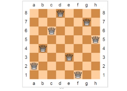
Eight queens puzzle is the problem of placing eight chess queens on an 8×8 chessboard so that no two queens attack each other. Thus, a solution requires that no two queens share the same row, column, or diagonal. The eight queens puzzle is an example of the more general n-queens problem of placing n queens on an n×n chessboard, where solutions exist for all natural numbers n with the exception of n=2 and n=3.

In computer programming, the solution to this problem is considered a classic involving problem-solving, algorithms, and data structures. This approach has several applications in scheduling, distributed systems, networking, etc.

There are two explicit solutions for n=4 and the solutions can be obtained in z^3 as follows:

In z^3, the user can use the NQUEEN function in several ways to get the solution, as well as explore and discover patterns associated with these solutions.

The result will be 92 solutions to 8 Queens problem, the first and last are given in the following:

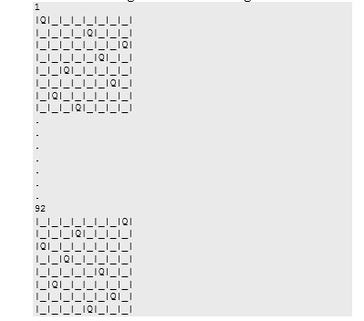
More interestingly, you can compute and get in a range of data values for different sizes as follows:

It scales-up easily, and consider sizes of chessboards with sizes 8..12.

204. $> NQUEENS(8..12)

The results of the above Example range from 352 solutions for 8 queens upto 14200 Solutions for 12 queens. In simpler cases, solutions could be sparse as follows.

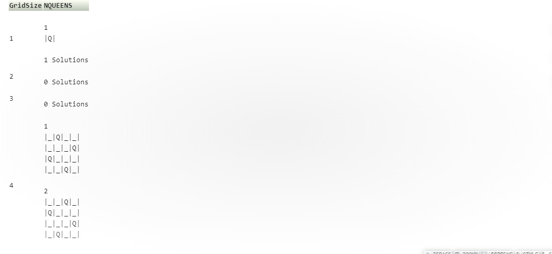
For practical purposes, the results become too large when it gets to a size of 19 queens.

Birthday Probability

In probability theory, birthday probability is a simple yet interesting problem. The history of this problem is obscure. Possibly, Harold Davenport or Richard von Mises proposed what we consider today to be the birthday problem.

This problem solves the probability of at least two of the n people in a room sharing a birthday. In a group of n people, there are 365n possible combinations of birthdays.

The simplest solution is to determine the probability of no matching birthdays and then subtract this probability from 1.

When n ≤ 365: $p(n)=1-{\dbinom {364}{365}}^{C(n,2)}=1-{\dbinom {364}{365}}^{\frac {n(n-1)}{2}}$

In a random group of 23 people, there is actually about a 50–50 chance that two of them will have the same birthday. Sample solutions for the following problems in z^3 are as follows:

This is known as the birthday paradox. In a room of 75 there’s a 99.9% chance of two people birth day matching.

In a group of 6 people, the following gives how many of them celebrate their birthday in the same month?

The decimal value is equivalent percentage value of 78%.

In a list of 40 people, it is 88%.

Towers Of Hanoi

The Tower of Hanoi puzzle was invented by the French mathematician Edouard Lucas in 1883. This puzzle is also known as Towers of Brahma.

The Tower of Hanoi problem is isomorphic to finding a Hamiltonian path on an n-hypercube.

Suppose three rods, as shown in the figure, and several disks with different sizes which can slide onto any rod.

The disks are arranged in ascending order of size on one rod, with the smallest one at the top in a stack, such that it makes a conical shape.

The objective of the game is to move all the disks onto a different pole with the following conditions:

• Only one disk can be moved at a time • Only the uppermost disk can be moved from any stack. • The smaller disk should always occupy the upper position of each stack at all times.

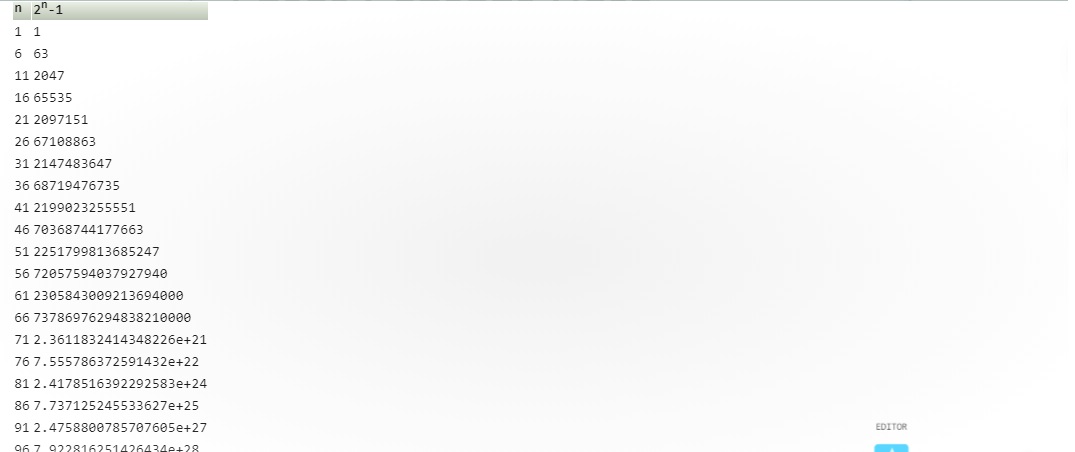
The puzzle can be solved in seven moves for three disks. The minimum number of moves required to solve a Tower of Hanoi puzzle is 2^n - 1, where n is the number of disk.

Hence the number of steps can be expected to increase rapidly, with the number of disks. Using z^3, number of steps to can be calculated for varying n:

When n=3, we expect 7 steps.

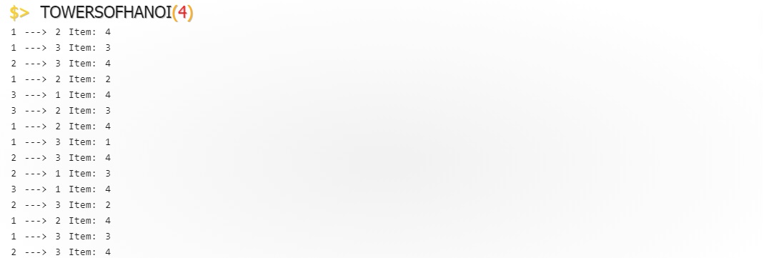
z^3 gives the following solution for 3 disks, which has 7 steps. At each step it also indicates the move made. Since the number of steps can be astronomical for a moderate number of disks, these calculations can exceed the capacity of the computer quite easily.

In z^3, the user can use the some other objects (instead of numbers) like:

More detailed solution showing step-by-step situation can also be obtained using z^3 as follows. Here, the disks are replaced by cat, dog and wolf, and the detailed moves to solve the problem is given by z^3.

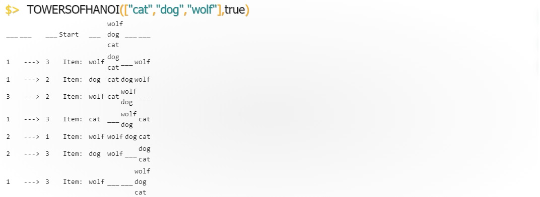The following Example indicates the number of steps for each number of disks ranging from 1 to 10, calculated after actually conducting the solution.

Floyds Triangle

Floyd’s triangle is the collection of natural numbers arranged in a right triangle to the left. It is named after Robert Floyd. Each line in Floyd’s triangle has one more element than the previous row, and has consecutive numbers from the left in each row. The nth row in the Floyd Triangle sums to ${\frac {n(n^{2}+1)}{2}}$, same as the constant of an n×n magic square.

In z^3, Floyd’s triangle displays as follows, with the first parameter indicating the number of rows to be displayed, and the second number indicating the limit of the natural number to be displayed.

Fractals-Mandelbrot

Compared to the Euclidean geometry, which has a long history of more than 2000 years, Fractal geometry is very new. Benoit Mandelbrot's famous book The Fractal Geometry of Nature was published relatively recently, in 1982. Nature is full of fractals, like trees, river networks, lightning bolts and blood vessels etc. Hence, fractal patterns tend to look extremely familiar and natural.

Fractals are infinitely complex patterns that are self-similar across different scales. This property is called “self-similarity”. Fractals form a never ending pattern, created by repeating a simple process over and over, in an ongoing feedback loop.

218. $> FRACTAL(20)

In z^3, user can get varying accuracy of fractals, by setting the parameter of the FRACTAL call.

The following call will create FRACTAL diagrams for an accuracy of 10, 100 and 1000. The quality of the generated fractal improves with the accuracy used, as evident from the generated examples given below.

Mandelbrot Set is the set of points in the complex plane with the sequence ( c , c² + c , (c²+c)² + c , ((c²+c)²+c)² + c , (((c²+c)²+c)²+c)² + c , ...), where the result does not approach infinity. The Julia Set is closely related to Mandelbrot Set.

The Mandelbrot Set is obtained from the quadratic recurrence equation:

$z_{n+1}={z_{n}}^{2}+c$, (with $z_{0}$=0),

where points c in the complex plane for which the computed value of $z_{n}$ does not tend to infinity.

The colors represent points that remain bounded within a limit for such recursive calls.

FDZ3()

FDZ3 gives the FRACTAL generated for $z_{n+1}={z_{n}}^{3}+c$.

Lissajous

Lissajous Curve is a parametric plot of the harmonic system. It is also called Bowditch Curves. This family of curves was investigated by Nathaniel Bowditch, an American mathematician in 1815, and later in more detail by Jules Antoine Lissajous in 1857.

Lissajous used sounds of different frequencies to vibrate a mirror. A beam of light reflected from the mirror, was allowed to trace patterns which depended on the frequencies of the sounds – in a setup similar to projectors used in today's laser light shows.

Lissajous figures often appeared as props in science fiction movies made during the 1950's. It has serious applications in physics, astronomy, and other sciences today.

Technically, Lissajous figure is the intersection of two sinusoidal curves, the axes of which are at right angles to each other. Mathematically, this translates to a Complex harmonic function: $x=Asin(at+\delta ),y=Bsin(bt)$

The appearance of a figure is highly sensitive to a/b, the ratio of a and b.

According to the ratio value, the shapes of the figures change in interesting ways.

For a a/b ratio=1, the figure is an ellipse.

For a=b, δ = π/2 radians, the figure is a circle.

For δ = 0, the figure is a line.

For a/b = 2, δ = π/4, the result is a parabola.

The Lissajous curve gets more complicated for other ratios, which are closed only if a/b is rational.

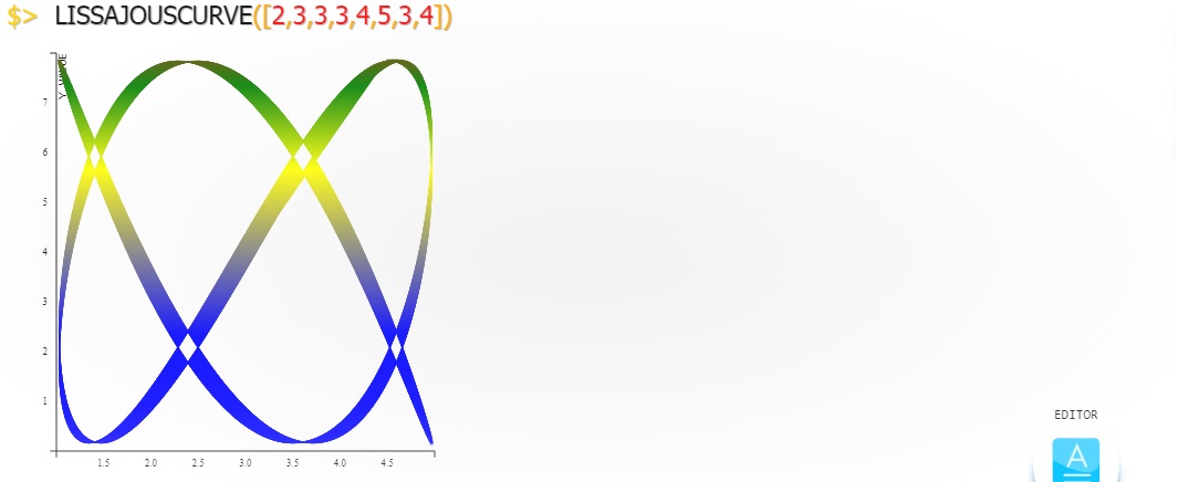
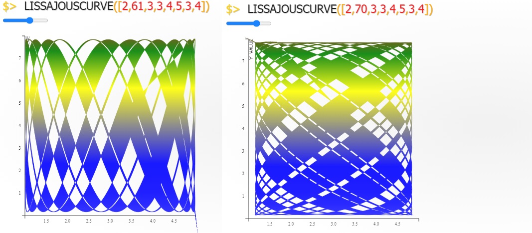
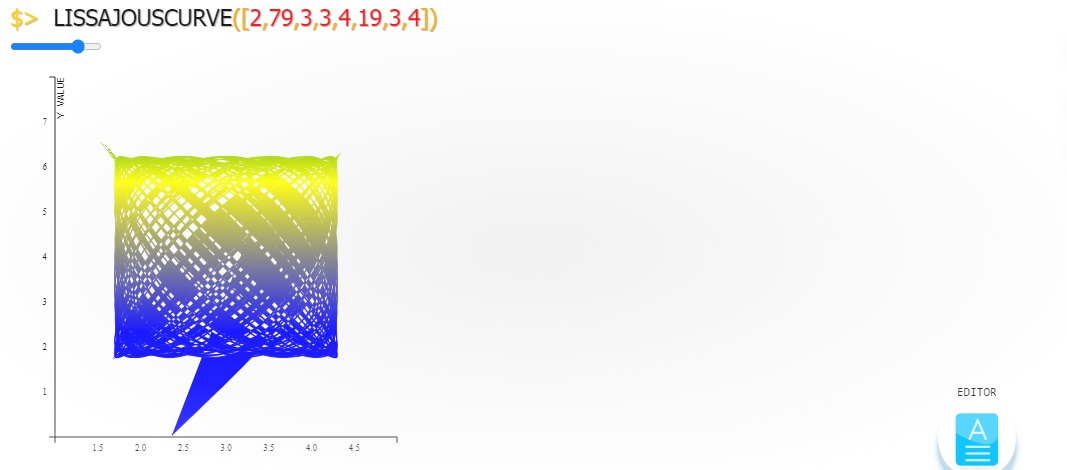
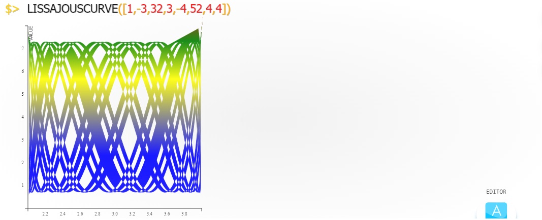
LISSAJOUSCURVE function can be given upto 8 parameters packed in a set indicating a1, b1, c1, d1, a2, b2, c2 and d2, or a string like "ellipse", "parabola" etc.

With the interactive parameter changing technique, right click on the parameter that you want to change on the ZOS display lines. Use the range controls that appear to generate a variety of such curves as given below.

LISSAJOUS Curves are fascinating regarding the types of curves you can generate by simply changing the parameters.

Graphing Data curve

A plot is used for representing a dataset graphically - usually showing the relationship between two or more variables. Graphs of functions are used in mathematics, sciences, engineering, technology, finance, and many other areas.

Two axes are using to plot a graph. The horizontal axis is called the x-axis and the vertical one is the y-axis. 1..10..0.008@COS .graph()

In z^3, user can also use multiple functions to plot a graph showing values from both: 226. $> 1..360@[DSIN,DCOS] .graph()

Financial Functions

A variety of functions are available in z^3. The functions generally follow the functions available in Spreadsheets, Databases, etc.

For example, PMT function finds the payment per period for a loan, based on constant payments and a constant interest rate.

The general syntax for this is:

$PMT(Rate,NoPaymentPeriods,PresentValue,FutureValue,Type)$

The Type parameter can be 0 or 1, to indicate the payment at the start of end of the period.

Now, we can really rev things up to analyze a variety of inputs with a single command.

Similarly, the future value of an annuity can be calculated using the FV function, given the rate, number of payment periods, payment per period, optional present value and a type flag indicating the payment to be done at the start or end of the period.

On the other hand, PV function gives the present value, for an optional future value. This can easily be followed by changing the parameters to try out different scenarios, such as changing the type parameter.

To find the number of days of in the coupon period that contains the settlement date, use the COUPDAYS function.

COUPDAYBS gives the number of days from the beginning of a coupon period until its settlement date.

COUPDAYSNC gives the number of days from the settlement date to the next coupon date.

Several functions also available in z^3 to calculate financial values, of which some are indicated below.

• XIRR - To calculate internal rate of return.

• IRR - To calculate the internal rate of return of a cash flow stream associated with an investment.

• MIRR - To find the value of the modified internal rate of return for a particular cash flows.

• XNPV - To find the net present value for a schedule of cash flows.

• NPV - To calculate the net present value of an investment.

• SYD - To find the depreciation of an asset for a given time period.

• EFFECT - To calculate the effective annual interest rate.

Combination of these financial functions with combinatorial arguments, provides the ability to do flexible analysis for a variety of inputs as below.

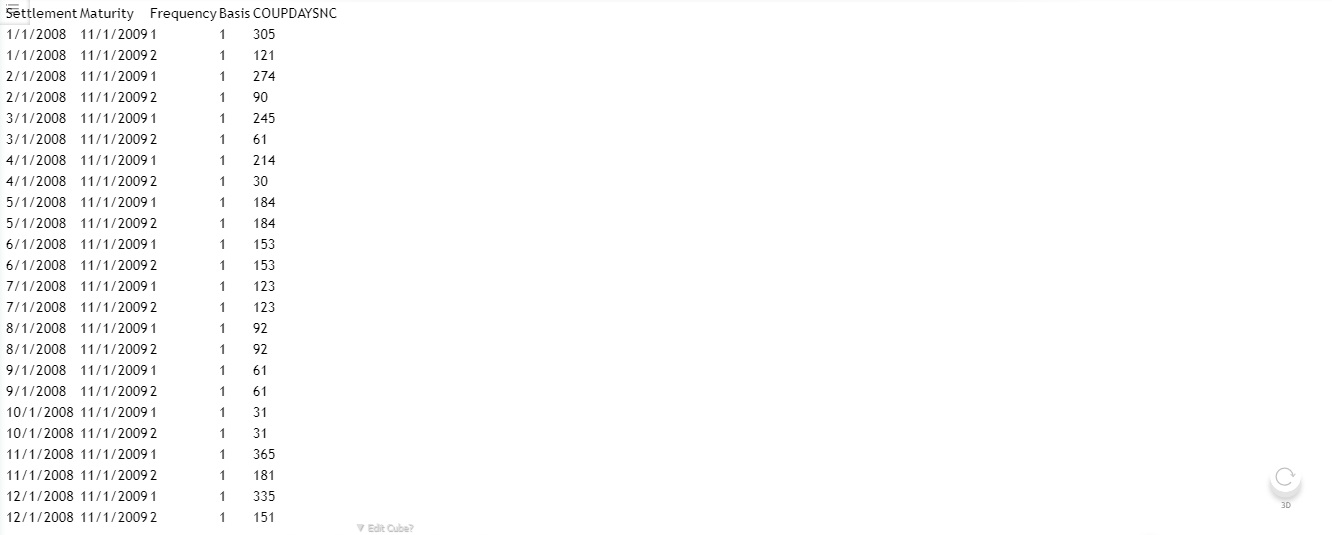
The above example shows the possibility of analysis by varying the parameters over ranges of dates,frequencies, etc. This can be a powerful analytical or teaching tool in professional and educational settings.

Listing of dates in a series can be achieved by the # operator for easy use in date and financial functions. DAYSINYEARTILLDATE(#2/2/2012-2/12/2012)

Statistical Functions:

In mathematics, statistics is the body of science that deals with the analysis, interpretation, presentation and organization of data. z^3 provides a large collection of statistical functions that perform most of the common Statistical calculations from simple min, max, mean, median and mode calculations to more complex Statistical Distribution and Probability tests, Distributions, Frequency, Rank, Deviation, Variance, Trend Lines, etc.

Using z^3, user can conduct a variety of Statistical Tests. These include Leven's test, Wilcoxon Signed Rank Test, F-Test, T-Test, Z-Test, Mann-WhitneyU test, Kruskal Wallis Test, Sign Test, Friedmann Test, Moods Median Test, Riemann Zeta test, etc. among many others.

Appendices

Appendix I Operators

The following operators are used in the z^3 language:

+, -, *, /, ^, %	Arithmetic Operators
|	Array Function and Creation Operator
.. , ...	Arithmetic and Geometric Series Creation
@	apply to
#	Series or Special Case Qualifier for Dates, Calci Cells, and Sequences, etc.
<<<	Member or Variable Assignment
()	Function Call
[]	Set Creation
{}	Object Set
[“key”]	Set Object Membership
.	Member Function Dereferencing
. mf	Member Function
.$(function, parameters)	Element-wise Function Application
.$$(function, parameters)	Row-wise Function Application
.$$$(function, parameters)	Column-wise Function Application
.$_(function, parameters)	Cumulative Function Application (all)

Appendix II: Simple Set and Objects

Set

Simple Set are declared using the conventional [ ] notation, and items are then accessed using the common [index] notation.

Associative Set/Objects

In z^3, associative set are distinct from simple set, in both declaration and qualification syntax.

Associative set can be declared using { } notation, with members within indicated using (:) as the separator between the member id and the value. While accessing such a member, conventional operator (.) is used to reference it.

In the following example all these characteristics are demonstrated elegantly as a data and a function are associated.

Appendix III: Javascript and z^3

z^3 uses Javascript as a backbone and provides full functionality and power of Javascript to pass through.

Using Set Member Functions

For example, any set, including matrices, can be operated on using any of the set member functions.

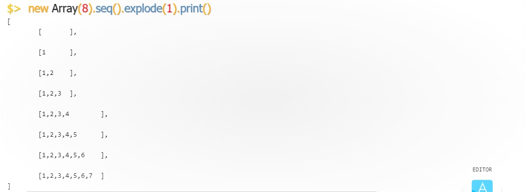
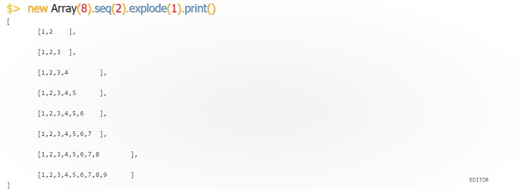
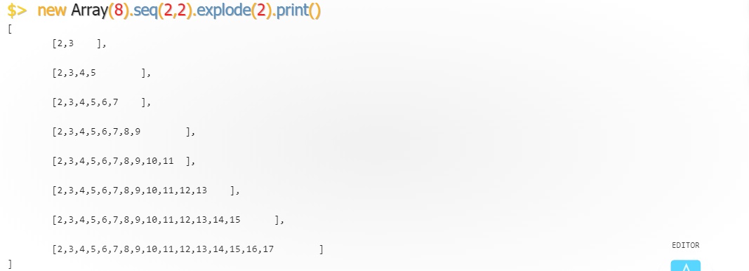
This can be triggered even with simple javascript commands as follows. Note the repeated application of additional member functions. In the following, .seq() fills a set with a sequence, and .explode() expands an element into a set having elements from 1 to that element.

An identity matrix of size 5 is generated, filled with random numbers and then cleared and filled with 3, and is printed below.

Appendix IV Series Generation

Creating series of items to be the input for further processing is a powerful aspect of z^3.

These can range from arithmetic series, geometric series, other prepacked series, alphabet series, and date series.

Arithmetic Series

<Start>..<end>..<interval>

notation is adopted for arithmetic series. e.g.:

Geometric Series

<Start>…<end>…<index>

notation is adopted for arithmetic series.

e.g.:

Prepacked Series

Several standard situations like angles in radians of degrees are indicated as below.

The terms can be composed using the pattern, (the numbers can be changed as you need), in a self-evident manner:

e.g.,

Date Series

A series of dates can be generated using # symbol followed by the data range. #<Start>-<End > Dates.

e.g.:

Alphabet Series

A series of letters can be generated using # symbol followed by the letter range. #<Start>-<End Letters. e.g.:

Appendix V Member Functions

The following is a listing of member functions for sets, strings, functions, objects and other key objects. By convention, member functions follow lowercase notation in general, while primary functions follow uppercase notation. The intellisense capability on the command-line assists users with listing of functions and arguments, simply by pressing Ctrl+Space using the keyboard. Set member functions are given under the Array object in the following table, in an interchangeable manner.

Array	$	Array of Functions
Array	$$	Array of Functions
Array	$$$	Array of Functions
Array	$$F	Array of Functions
Array	$A	Parameter
Array	$C	Column Array to apply, Function
Array	$CELLS	Array of Functions, Optional Parameters
Array	$d
Array	$diag
Array	$dth
Array	diagonal
Array	$R	Row Array to apply, Function
Array	$X
Array	$x
Array	_$
Array	$_
Array	ac	ColCount
Array	accumulate	Total
Array	accumulatewith	CumulateFunction, CurrentResult
Array	across	OtherArray, Function
Array	add	Thing
Array	addcolumn	NumberOfColumns
Array	addrow	NumberOfRows
Array	addsequence	InFront, StartFrom, OptionalSequenceArray
Array	adjoint
Array	aggregate	Columns,Function, Params
Array	allslices	SliceSize
Array	any	Count
Array	appendfunction	Function
Array	ar
Array	async	Iterator, CallBack
Array	atindex	List of indices
Array	atnode	Function, SubtractByArray, ScaleByArray, DoNotShowIndices
Array	backward	Function, StartValue
Array	bindcolumn
Array	branch	SomeOnlyMatches
Array	branchvalues	SomeOnlyMatches
Array	buckets
Array	bykey
Array	c	Columns
Array	calci
Array	head
Array	cartesianproduct	IsWithoutFlatten
Array	cdr
Array	cell	Row, Column, Width, Height
Array	cells	Row, Column, Width, Height
Array	checktype	TypeArray, ForceCheckOnVariables
Array	chunks	ChunkSize
Array	ci
Array	clean	Expression, ReplaceWith
Array	clear	FillWith
Array	clearcopy	FillWith
Array	clone
Array	colconcat	AnotherArray
Array	colcount
Array	collect
Array	collectasvector
Array	collectwhile
Array	collectwhileasvector
Array	column	SomeColumns
Array	columnconcat	AnotherArray
Array	columns	SomeColumns
Array	compare
Array	concatall	LimitArray, IncludeEdges
Array	converge	Function, NumberOfIterations, Accuracy, Converge
Array	copy
Array	core
Array	count	FirstLevelOnly
Array	crosstab	RowSet, ColSet,PageSet,DataSet
Array	cube
Array	cumcolumn
Array	cumcolumns
Array	cumcolumnswith
Array	cumcolumnwith
Array	cumrow
Array	cumrows
Array	cumrowswith
Array	cumrowwith
Array	cumulate
Array	data
Array	dc	Which
Array	deal	Within, ManyInEach
Array	deepcopy
Array	deletecolumn	Which
Array	deleterow	Which
Array	det	Array
Array	determinant	Array
Array	dim	Dimensions
Array	div	OtherNumber
Array	divide	OtherNumber
Array	dr	Which
Array	dropwhile
Array	dropwhileasvector
Array	eighteenth	SomeCount
Array	eighth	SomeCount
Array	eleventh	SomeCount
Array	equal	Array, CheckLength, StartFrom
Array	equalvalues	Array, CheckLength, StartFrom
Array	eval
Array	except	Indices
Array	exec	Parameters
Array	explode	StartIndex, By, RecurseTillLevel
Array	extract	column list
Array	few	IncludeHeader
Array	fifteenth	SomeCount
Array	fifth	SomeCount
Array	fillwith	Numbers
Array	filtermatches	MatchIdenticalMatrix, OnlyMatches
Array	filteroncolumn	Condition, ExtractColumns, FilterOnColumn
Array	filteroncondition	TakeDropOrAllFlag, Function, Parameter
Array	filteronrow	Condition, ExtractRows, FilterOnRow
Array	findcellref	Values
Array	first	SomeCount
Array	firstelement	SomeCount
Array	firsthalf
Array	fixat	Index, Fix
Array	fjoin	HeadLength, JoinString
Array	flatten
Array	flip	IncludeHeader
Array	flipparts
Array	fold	AtFoldValue, AtReverseFoldValue
Array	foldl	Function, StartSeed
Array	foldr	Function, StartSeed
Array	forward	Function, StartValue
Array	fourteenth	SomeCount
Array	fourth	SomeCount
Array	fourths
Array	funcjoin	HeadLength, FindString, FirstString, MidString, LastString
Array	graph	Mode
Array	half
Array	halves
Array	head
Array	headings
Array	hundredth	SomeCount
Array	i	PreviousArray
Array	ic	Functions
Array	ids
Array	implode	RecurseTillLevel
Array	include
Array	indices	Function, SubtractByArray, ScaleByArray, DoNotShowIndices, RowArray
Array	injoin	JoinWith
Array	inner	InnerSize
Array	insert	Value, AfterLastFlag
Array	insertcolumn	Index, NumberOfColumns
Array	insertrow	Index, NumberOfRows
Array	inverse	Array
Array	is	Thing, IsNot
Array	is1d
Array	is2d
Array	isFalse
Array	isnotnull
Array	isnull
Array	isTrue
Array	joincolumnswith	ArrayOfJoinCharacters, IsRepeat
Array	joinrowswith	ArrayOfJoinCharacters, IsRepeat
Array	joinwith
Array	last
Array	lastelement
Array	make1to2d
Array	makekeyarray	Recursive
Array	maplist	fun
Array	mapper	Function
Array	maprow	Function
Array	match	Expression
Array	matchcolumn	Expression, Column
Array	matchindex	Expression, IndexThenFromMatch
Array	matchrow	Expression, Row
Array	matchvalue	Expression, IndexThenFromMatch
Array	merge	OtherArray, Function
Array	mergecolumns	OtherArray
Array	mergerows
Array	mid	From, Count
Array	millionth	SomeCount
Array	mod	Thing
Array	multiply	Thing
Array	nicejoin	JoinString, EndString, SubArrayString
Array	nineteenth	SomeCount
Array	nineth	SomeCount
Array	nodeindex
Array	notinclude
Array	notwithinlimits	LimitArray, IncludeEdges
Array	nth	Nth, Count
Array	ntimes	Function, NumberOfIterations, Accuracy, Converge
Array	nullifyobjects	Recursive
Array	numbers	ForceCheckOnVariables
Array	objects	List of Items
Array	of	elements
Array	op
Array	otherthan	ArrayWithElementsToExclude
Array	outer	OuterSize
Array	pack
Array	pad	Length, PadString
Array	pair	Value, OnRight
Array	pairmatch	AtFoldValue, AtReverseFoldValue, StartFrom
Array	partitiononcondition	TakeDropOrAllFlag, Function, Parameter
Array	parts	NumberOfParts, SpecificPart
Array	pastefolds	MidOnly
Array	pick	PickMaskArray
Array	pieces	Width, Function
Array	pip	PathIndexArray, Length, PassThroughFunction,UseClone
Array	pipall	ExceptIndexUpto, MarkSliced
Array	pipallwithslice	ExceptIndexUpto, MarkSliced
Array	prefix	Prefix
Array	primitives
Array	print	Trimmed, TabLevel
Array	rand
Array	random
Array	raw
Array	remove	List of Elements
Array	removebyval	Value
Array	removeindices
Array	repeatntimes	Function, NumberOfIterations, Accuracy, Converge
Array	replace	ExpressionArrayOrValues, ReplaceWith
Array	replicate	Count
Array	rest	Start, Count
Array	reverse	Function, StartValue
Array	reverselevel	Level
Array	reversepip	SomeExceptIndexUpto, SomeMarkSliced
Array	reversesort	Function
Array	rotate	NumberOfSteps
Array	rotatecolumns	NumberOfSteps
Array	rotaterows	NumberOfSteps
Array	row
Array	rowconcat	OtherArray
Array	rowcount
Array	rowlengths	Function
Array	rowpush	OtherArray
Array	rslice	Begin, End
Array	second	SomeCount
Array	secondhalf
Array	seq	StartIndex, By
Array	set
Array	setaxis	Axis, ColumnValues
Array	setcolumn	Column, ColumnValues
Array	setheadings	Header List as Parameters
Array	setrow	Row, Array
Array	seventeenth	SomeCount
Array	seventh	SomeCount
Array	shiftlevel	Level, NumberOfTimes
Array	shuffle
Array	sixteenth	SomeCount
Array	sixth	SomeCount
Array	size
Array	slices	SliceExpression
Array	some	callback[, thisArg
Array	sortbykey
Array	specialprint	Trimmed,TabLevel
Array	spliteach	SplitExpression, RetainSplitterAlsoInResult
Array	splitwhile
Array	splitwhileasvector
Array	stringlist
Array	subtract	Thing
Array	suchthat
Array	suchthatasvector
Array	suffix	suffix
Array	table
Array	tablelookup	RowValueMatch, ColumnValueMatch
Array	tail
Array	takewhile
Array	takewhileasvector
Array	tenth	SomeCount
Array	third	SomeCount
Array	thirds
Array	thirteenth	SomeCount
Array	thousandth	SomeCount
Array	transpose	IncludeHeader
Array	truefalse	IsCheckTrueFunctionList, IsCheckFalseFunctionList, DoFlattenFirst
Array	twelfth	SomeCount
Array	twentieth	SomeCount
Array	uncrosstab	UptoColumn
Array	unimplode
Array	unimplodeleaf
Array	unzip	OtherArray
Array	value	Function
Array	where	Term
Array	withinlimits
Array	X$	SomeArray
Array	xy	Function, OffsetArray, ScaleArray,GiveIndicesAlso,DoCentering
Array	xypanel	FunctionArray, OffsetArray, ScaleArray, GiveIndicesAlso
Array	zero	ValueInstead, PreserveStructure
Array	zip	OtherArray

How to work with zcubes

Here are the links to help you on working with ZCubes and learn more about ZCubes features.

http://wiki.zcubes.com/Learn_ZCubes

www.zcubes.com Do It All!